Pathways Visualisation

Author

Affiliation

Alejandra Escobar

MGnify team at EMBL-EBI

This is a static preview

You can run and edit these examples interactively on Galaxy

MGnifyR is a library that provides a set of tools for easily accessing and processing MGnify data in R, making queries to MGnify databases through the MGnify API. The benefit of MGnifyR is that data can either be fetched in tsv format or be directly combined in a phyloseq object to run an analysis in a custom workflow.

This is an interactive code notebook (a Jupyter Notebook). To run this code, click into each cell and press the ▶ button in the top toolbar, or press shift+enter.

Pathways Visualisation

In this notebook we aim to demonstrate how the MGnifyR tool can be used to fetch functional annotation results generated through the MGnify metagenomic analyisis pipelines.
Then we show how to generate the pathways visualization using Pathview in R with the following input data:

Annotated functional genes MGnify
Annotated metabolic compounds Metabolights

Introduction
- Minimal example 1. Fetching KEGG orthologs and modules tables from MGnify
- Minimal example 2. Accessing to KEGG pathways info using the KEGGREST API
Part 1. Drawing presence/absence of KOs for one metagenomic sample
Part 2. Comparing groups of samples, drawing KOs abundance
Part 3. Plotting presence/absence of KOs and metabolites for one sample
References

# Loading libraries:
suppressMessages({
    library(ALDEx2)
    library(data.table)
    library(dplyr)
    library(IRdisplay)
    library(KEGGREST)
    library(MGnifyR)   
    library(pathview)
    library(tidyjson)
})
    
#display_markdown(file = 'assets/mgnifyr_help.md')

# Setting tables and figures size to display (these will be reset later):
options(repr.matrix.max.cols=150, repr.matrix.max.rows=500)
options(repr.plot.width=4, repr.plot.height=4)

# Setting up functions
collect_pathways <- function(ids_list) {
    pathways = list()
    for (id in ids_list) { 
        current_pathway = as.list(keggLink("pathway", id))
        for (index in grep("map", current_pathway)) {        
            clean_id = gsub("*path:", "", current_pathway[index])
            # Discarding chemical structure (map010XX), global (map011XX), and overview (map012XX) maps
            prefix = substring(clean_id, 1, 6)
            if(is.na(match("map010", prefix)) & is.na(match("map011", prefix)) & is.na(match("map012", prefix)) ){
                pathways = append(pathways, clean_id)
            }
        }
    }
    return(pathways)
}

# Create your session mgnify_client object
mg = mgnify_client(usecache = T, cache_dir = '/home/jovyan/.mgnify_cache')

Introduction

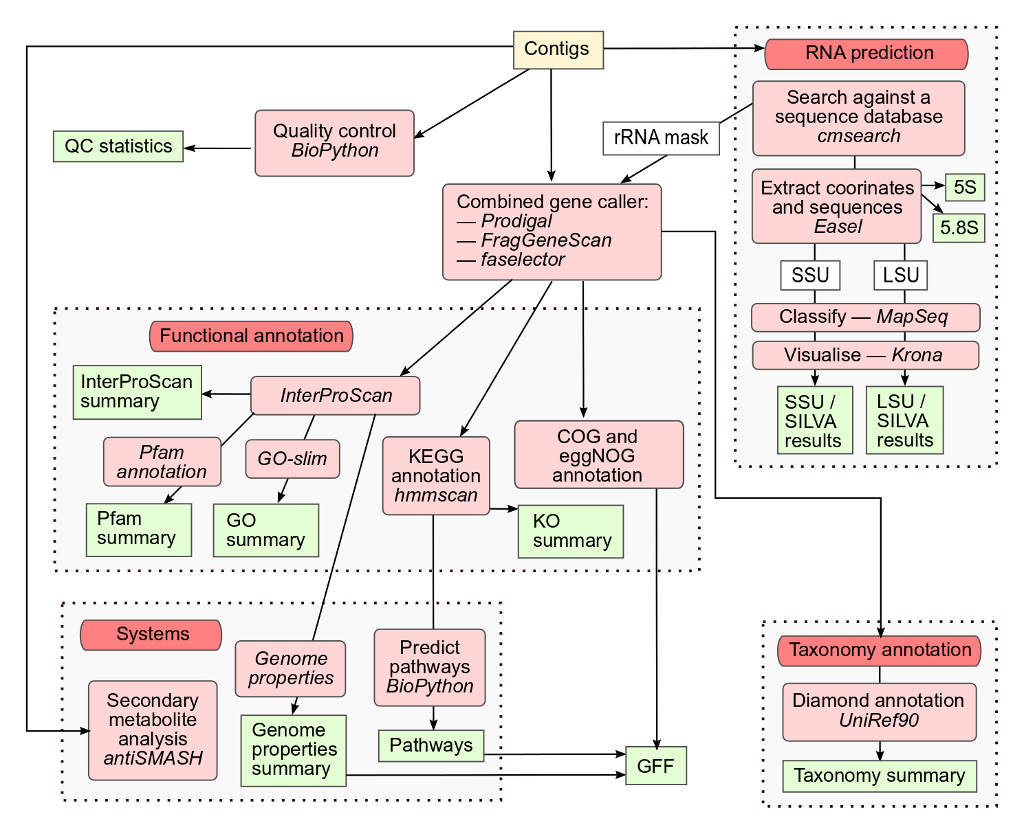
The goal of this notebook is to demonstrate how to create KEGG pathway maps to visualise metabolic potential and metabolite production in metagenomic samples. We will use metabolic pathways annotated at the gene level by assigning a KEGG Orthology (KO) to putative protein sequences. These results are generated through the MGnify v5.0 pipeline for metagenomic assemblies, as shown in the workflow schema below. We will also use the completeness estimation of KEGG modules available in the MGnify web portal. Consider that modules completeness is determined by the shortest possible path which contains the essential steps for the pathway; therefore, even if 100% completeness is achieved, there can still be gaps.

The KEGG (Kyoto Encyclopedia of Genes and Genomes) database is a collection of biological databases, including genetic and metabolic pathways, diseases and drugs, protein-protein interactions, and gene expression. We use the KEGG database to make connections between genes and their biological functions, and define pathways containing the functions to be used as a resource for systems biology.

Some key concepts we will use in this notebook are:

KEGG Orthologs (KO): Orthologs are genes in different species that evolved from a common ancestral gene and typically retain similar functions. KEGG Orthologs are a set of manually curated genes and proteins grouped into categories based on their functional similarities, particularly their roles in biological pathways and molecular functions. KEGG Orthologues IDs are unique and always starts with the letter ‘K’ (uppercase) followed by 5 numbers.
KEGG Modules: Modules are clusters of related genes that are involved in a specific biological process or pathway. KEGG modules IDs starts with ‘M’ followed by 5 numbers.
KEGG Pathways: Pathways are sets of interconnected biochemical reactions that form a chain leading from an initial reactant to a final product. KEGG pathways provide a high-level overview of the major metabolic pathways in an organism, while KEGG modules provide a more detailed view of the genes and reactions involved in a specific pathway. The IDs of manually drawn reference pathway starts with the word ‘map’ followed by 5 numbers. Another pathways prefix you will se in the notebook is ‘ko’ for reference pathway highlighting KO.

For a better display of results, in this notebook we are not using as templates chemical structure (map010XX), global (map011XX), and overview (map012XX) maps.

Alt Text — Mgnify assembly analysis pipeline v5.0

In the following sections of this introduction you will find a couple of simplest minimal examples on the main functions we will use to fetch and format the input tables for KEGG pathways visualization.

Minimal example 1. Fetching KEGG orthologs and modules tables from MGnify

MgnifyR has pre-built functions to retrieve data from MGnify databases. The mgnify_retrieve_json function can be used to access results that are not available in tabular format. In this notebook we will fetch the pathways annotation and pathways completeness tables generated by the latest version of the MGnify analysis pipeline in json format and reformat into dataframes to easily manipulate the data.

Example on how to fetch the KOs counts table for one sample having the analysis accession MGYA00636312:

ko_json = mgnify_retrieve_json(mg, path = 'analyses/MGYA00636312/kegg-orthologs')
ko_data = as.data.frame(ko_json %>% spread_all)[ , c("attributes.accession", "attributes.count")]

head(ko_data, 3)

And we can also fetch the modules completeness table for the same sample using the following code:

ko_comp_json = mgnify_retrieve_json(mg, path = 'analyses/MGYA00636312/kegg-modules')
ko_comp = as.data.frame(ko_comp_json %>% spread_all)[ , c("id", "attributes.completeness")]

head(ko_comp, 3)

Minimal example 2. Accessing to KEGG pathways info using the KEGGREST API

KEGGREST is a powerful tool with multiple functions to access and utilize data from KEGG databases. We can use KEGGREST to map between IDs in different databases and to find pathways associated with a module, orthologue, or compound. To display the list of KEGG databases we can query, you can run listDatabases() command.

With keggLink function we can find the ID of the pathways to use as template to draw the module of methane production from CO2 (M00567). We find that the module M00567 is present in 4 possible pathways.

as.list(keggLink("pathway", 'M00567'))

Using keggFind to find all the KOs associated to the Methyl-coenzyme M reductase (EC 2.8.4.1)

as.list(keggFind("ko", '2.8.4.1'))

Part 1. Drawing presence/absence of KOs for one metagenomic sample

For Parts 1 and 2 of this notebook, we will use MGnify results generated for two studies: 1. Metagenomes of bacteria colonizing the gut of Apis mellifera and Apis cerana from Japan (MGYS00006180). 2. Gut microbiota of Switzerland honeybees (MGYS00006178).

The original analysis based on viral communities can be found in the Bonilla-Rosso et al., publication.

1.1. Fetching data from MGnify

Fetching the analysis accession list using the study accessions.

all_accessions = mgnify_analyses_from_studies(mg, c('MGYS00006180','MGYS00006178'))
all_metadata = mgnify_get_analyses_metadata(mg, all_accessions)

Keeping just the first analysis accession to fetch the kegg orthologs count table from the MGnify API and transform from JSON to matrix.

accession = head(all_accessions, 1)
ko_loc = paste0('analyses/',accession,'/kegg-orthologs')

ko_json = mgnify_retrieve_json(mg, path = ko_loc)
ko_data = as.data.frame(ko_json %>% spread_all)[ , c("attributes.accession", "attributes.count")]
ko_data = data.frame(ko_data, row.names=1)
colnames(ko_data)[1] = 'counts'
ko_matrix = data.matrix(ko_data)

head(ko_matrix, 3)

1.2. Selecting pathways

We are going to draw metabolic pathways for essential metabolism of carbohydrates plus fructose and manose metabolism, which is non-essential:

Glycolysis/Gluconeogenesis (00010)
Citric Acid (TCA) Cycle (00020)
Pentose Phosphate Pathway (00030)
Fructose and manose metabolism (00051)

to_draw = c('map00010', 'map00020', 'map00030', 'map00051')

1.3. Ready to draw!

As we are plotting absence/presence, we set the number of bins = 2, the scale in one direction, and use 1 as limit. You will see some ‘Note’ and ‘Info’ messages, don’t panic, it is pathview normal behaviour.

for (p in to_draw) {
    nude_id =  gsub("map", "", p)
    pathview(gene.data = ko_matrix, 
             species = "ko", 
             pathway.id = nude_id, 
             bins=c(2, 2), 
             both.dirs = FALSE, 
             limit = c(1,1), 
             mid = c("#ffffff" , "#ffffff"), 
             high = c("#02b3ad" , "#02b3ad")
    )
}

Cleaning the working directory.

if(!dir.exists("output_plots")){
    dir.create("output_plots")
    dir.create("output_plots/single_sample")
}

file.copy(from=list.files(pattern="./*pathview.png"), to="./output_plots/single_sample/", overwrite = TRUE)

png_files = list.files(path = ".", pattern = "*.png")
xml_files = list.files(path = ".", pattern = "*.xml")
files = c(png_files, xml_files)
unlink(files)

This is one example of Pathview outputs. The rest of the generated figures are stored at output_plots/single_sample/ directory. You can explore the files by clicking on them at the left-side panel.

display_png(file='./output_plots/single_sample/ko00030.pathview.png')

Part 2. Comparing groups of samples, drawing KOs abundance

In this part of the notebook we use the whole list of accessions for both studies (MGYS00006180 and MGYS00006178). After integrating the KO’s tables, we run Aldex2 to find differentially abudant genes with KO annotation between honeybees from Japan and Switzerland, and we use the effect as scale to plot the pathways with the highest number of differentially abundant KOs. Consider that steps involving fetching KO tables and KEGGREST queries can take few minutes to run.

2.1. Fetching KO tables from MGnify

Generating condition labels.

accession_alias = subset(all_metadata, select = c('analysis_accession', 'study_attributes.accession'))

cond_list = list()
for (study_id in accession_alias$'study_attributes.accession') {
    if (study_id == 'MGYS00006180') {
        cond_list = append(cond_list , 'Japan')
    } else {
        cond_list = append(cond_list , 'Switzerland')
    }
}
accession_alias$condition = cond_list

table(unlist(accession_alias$condition))

Selecting randomly 15 samples from each location to speed up the downstream analysis.

set.seed(123)
grouped_df = accession_alias %>% group_by(condition)
random_sample = grouped_df %>% sample_n(size = 15, replace = FALSE)

Download and integrate KO counts tables. We will discard any sample having zero genes with KO annotation. This step takes around 3 minutes to complete.

# Saving KO tables as a list of dataframes
samples_list = random_sample$'analysis_accession'
list_of_dfs = list()
for (accession in samples_list) {
    ko_loc = paste0('analyses/',accession,'/kegg-orthologs')
    ko_json = mgnify_retrieve_json(mg, path = ko_loc)
    ko_data = as.data.frame(ko_json %>% spread_all)[ , c("attributes.accession", "attributes.count")]
    colnames(ko_data) = c('ko_id', accession)
    list_of_dfs = append(list_of_dfs, list(ko_data)) 
}

# Integrating all dataframes into a single dataframe
integrated_df = list_of_dfs[[1]]
for (i in 2:length(list_of_dfs)){
    integrated_df = merge(integrated_df,list_of_dfs[[i]], all = T)
}

## Cleaning the integrated table
# Using the KO id column as row names
row.names(integrated_df) = integrated_df$ko_id
integrated_df$ko_id = NULL

# Converting NA to zero 
integrated_df[is.na(integrated_df)] = 0

# Discarding samples that KOs abundance sum = 0
integrated_df = integrated_df %>% select_if(is.numeric) %>% select_if(~ sum(. != 0) > 0)

head(integrated_df, c(3, 2))

Reformating the condition label according with the KOs dataframe.

sorted_conds = list()
for (sample in colnames(integrated_df)) {
    match = accession_alias[accession_alias$analysis_accession %in% sample,]$condition
    cond = paste(match, collapse = "")
    sorted_conds = append(sorted_conds, cond)    
}
vector_conds = unlist(sorted_conds)

table(vector_conds)

2.2. Generating differentially abundance count tables

Running Aldex step. It takes 2 minutes to complete.

x.all = aldex(integrated_df, 
              vector_conds, 
              mc.samples=128, 
              test="t", 
              effect=TRUE, 
              include.sample.summary=FALSE, 
              denom="all", 
              verbose=FALSE
        )

head(x.all, 3)

The column effect in the above output (x.all table) contains the log ratio of the sample mean to the reference mean. A positive effect indicates that the sample mean is greater than the reference mean, while a negative effect indicates that the sample mean is lower than the reference mean. In this example, Japan group is used as reference. We will generate now the matrix of KO-effect for plotting.

ko_matrix = data.matrix(subset(x.all, select = c('effect')))

head(ko_matrix, 3)

Plotting the effect size (effect) and difference (diff.btw) to show an overview of differentially abundant functions. Two type of P-value results from the Welch’s t test are shown: In blue marks the expected P-value; in red marks the expected Benjamini-Hochberg corrected P-value. The threshold line indicates P-value = 0.05.

options(repr.plot.width=10, repr.plot.height=8)

# Effect size plot
par(mfrow=c(1,2))
plot(x.all$effect, 
    x.all$we.ep, 
    log="y", 
    cex=0.7, 
    col=rgb(0,0,1,0.2),  # Blue marks for expected P value of Welch’s t test
    pch=19, 
    xlab="Effect size", 
    ylab="P value", 
    main="Effect size plot")
points(x.all$effect, 
    x.all$we.eBH, 
    cex=0.7, 
    col=rgb(1,0,0,0.2), # Red marks for expected Benjamini-Hochberg corrected P value of Welch’s t test
    pch=19)
abline(h=0.05, lty=2, col="grey")
legend(-0.5,0.0005, legend=c("P value", "BH-adjusted"), pch=19, col=c("blue", "red"))

# Volcano plot
plot(x.all$diff.btw, 
    x.all$we.ep, 
    log="y", 
    cex=0.7, 
    col=rgb(0,0,1,0.2), # Blue marks for expected P value of Welch’s t test
    pch=19, 
    xlab="Difference", 
    ylab="P value", 
    main="Volcano plot")
points(x.all$diff.btw, 
    x.all$we.eBH, 
    cex=0.7, 
    col=rgb(1,0,0,0.2), # Red marks for expected Benjamini-Hochberg corrected P value of Welch’s t test
    pch=19)
abline(h=0.05, lty=2, col="grey")
legend(-2,0.0005, legend=c("P value", "BH-adjusted"), pch=19, col=c("blue", "red"))

Reporting features detected by the Welchs’ or Wilcoxon test individually (blue) or by both (red).

options(repr.plot.width=8, repr.plot.height=8)

found.by.all <- which(x.all$we.eBH < 0.05 & x.all$wi.eBH < 0.05)
found.by.one <- which(x.all$we.eBH < 0.05 | x.all$wi.eBH < 0.05)

plot(x.all$diff.win, x.all$diff.btw, pch=19, cex=1, col=rgb(0,0,0,0.3),
 xlab="Dispersion", ylab="Difference")
points(x.all$diff.win[found.by.one], x.all$diff.btw[found.by.one], pch=19,
 cex=1, col=rgb(0,0,1,0.5))
points(x.all$diff.win[found.by.all], x.all$diff.btw[found.by.all], pch=19,
 cex=1, col=rgb(1,0,0,1))
abline(0,1,lty=2)
abline(0,-1,lty=2)

2.3. Selecting pathways to draw

We will use the union of both testing methods (Welchs’ or Wilcoxon) to find the pathways with differentially abundant KOs.

kos_list = list()
for (index in found.by.one){
    current_ko = rownames(x.all)[index]
    kos_list = append(kos_list, current_ko)
}

ko_pathways = collect_pathways(kos_list)

head(ko_pathways)

Finding the pathway with the highest number of significant KOs.

pathways_counts = list()
for (path_element in ko_pathways) {
    if (path_element %in% names(pathways_counts)) {
        new_value = pathways_counts[[path_element]] + 1
        pathways_counts[path_element] = new_value       
    } else {
        pathways_counts[path_element] = 1 
    }
}

top_to_plot = names(tail(pathways_counts[order(unlist(pathways_counts))], 1))
top_to_plot

2.4. Drawing pathways!

For this type of data, values range from -1 to 1, with both negative and positive fractions. We use both directions when plotting.

for (p in top_to_plot) {
    nude_id =  gsub("map", "", p)
    pathview(gene.data = ko_matrix, 
        species = "ko", 
        pathway.id = nude_id, 
        both.dirs = TRUE, 
        low = c("#bd066b", "#bd066b"),  
        mid = c("#c9c9c9" , "#c9c9c9"), 
        high = c("#02b3ad" , "#02b3ad")
    )
}

Cleaning the working directory.

if(!dir.exists("output_plots/comparative")){
    dir.create("output_plots/comparative")
}

file.copy(from=list.files(pattern="./*pathview.png"), to="./output_plots/comparative/", overwrite = TRUE)

png_files = list.files(path = ".", pattern = "*.png")
xml_files = list.files(path = ".", pattern = "*.xml")
files = c(png_files, xml_files)
unlink(files)

This is the Pathview output stored at output_plots/comparative/ directory.

display_png(file='./output_plots/comparative/ko00860.pathview.png')

Part 3. Plotting presence/absence of KOs and metabolites for one sample

For this part of the notebook we will use public data of the study An untargeted metabolomics approach to characterize dissolved organic matter in groundwater of the Samail Ophiolite. Metatranscriptomics (RNA-Seq) raw-reads are available at the ENA under the accession PRJNA560313. Analysis results are available on MGnify under the study accession MGYS00006297, and compound data can be found on Metabolights under the accession MTBLS6081.

3.1. Fetching KOs table from MGnify

As we are using only one sample, we will fetch metadata and the KO table for that sample directly from MGnify.

sample = 'MGYA00652853'
metadata = mgnify_get_analyses_metadata(mg, sample)
mgnify_sample = metadata$'sample_sample-name'
mgnify_sample

ko_loc = paste0('analyses/',sample,'/kegg-orthologs')

ko_json = mgnify_retrieve_json(mg, path = ko_loc)
ko_data = as.data.frame(ko_json %>% spread_all)[ , c("attributes.accession", "attributes.count")]
ko_data = data.frame(ko_data, row.names=1)
colnames(ko_data)[1] = 'counts'

# Transforming kos matrix into a named vector
ko_values = ko_data$'counts'
ko_names = rownames(ko_data)
ko_vector = setNames(ko_values, ko_names)

head(ko_vector, 3)

Find the pathways with at least 10 genes. This step takes 3 min to run.

ko_pathways = collect_pathways(ko_names)

pathways_counts = list()
for (path_element in ko_pathways) {
    if (path_element %in% names(pathways_counts)) {
        new_value = pathways_counts[[path_element]] + 1
        pathways_counts[path_element] = new_value       
    } else {
        pathways_counts[path_element] = 1 
    }
}
top_genes_pathways = names(pathways_counts)[sapply(pathways_counts, function(x) x > 9)]
print(length(top_genes_pathways))
#print(top_genes_pathways)

3.2. Fetching and formatting metabolites data

We will fetch the samples table s_MTBLS6081.txt and the compounds table m_MTBLS6081_LC-MS_negative_reverse-phase_metabolite_profiling_v2_maf.tsv from the Metabolights database using the url and save them on files with shorter names.

# Downloading the metabolites samples table
url = 'https://www.ebi.ac.uk/metabolights/ws/studies/MTBLS6081/download/39846581-6c64-4e09-99dd-74cb05921f85?file=s_MTBLS6081.txt'
destfile = 's_MTBLS6081.txt'
download.file(url, destfile = destfile, method = "auto")

# Downloading the compounds table
url = 'https://www.ebi.ac.uk/metabolights/ws/studies/MTBLS6081/download/39846581-6c64-4e09-99dd-74cb05921f85?file=m_MTBLS6081_LC-MS_negative_reverse-phase_metabolite_profiling_v2_maf.tsv'
destfile = 'm_MTBLS6081.tsv'
download.file(url, destfile = destfile, method = "auto")

Finding the sample ID corresponding to MGnify results on the metadata table

metadata_comp = read.table("s_MTBLS6081.txt", header = TRUE, sep = "\t")
metabolights_sample = metadata_comp[grepl(mgnify_sample, metadata_comp$'Source.Name'), ]$'Sample.Name'
print(c(mgnify_sample, metabolights_sample))

Parsing and formating the metabolites table

compound_data = read.table("m_MTBLS6081.tsv", header = TRUE, sep = "\t", comment.char = "|", quote = "") 
head(compound_data, 3)

# Keeping rows with CHEBI id
chebi_compound = compound_data[grepl("CHEBI", compound_data$database_identifier), ]

# Keeping data for the sample of interest only
chebi_compound = subset(chebi_compound, select = c('database_identifier', metabolights_sample))

# Discarding rows with abundance = 0
compound_clean = chebi_compound[chebi_compound[, 2] != 0, ]

head(compound_clean, 3)

Transforming CHEBI ids into KEGG compound IDs. To speed up this step, instead of using KEGGREST, we are going to use a relational table of IDs available at the FTP site of the EBI public databases.

# Downloading the relational table
url = 'https://ftp.ebi.ac.uk/pub/databases/chebi/Flat_file_tab_delimited/database_accession.tsv'
destfile = 'chebi2kegg.tsv'
download.file(url, destfile = destfile, method = "auto")

# Reading the table
chebi2kegg_df = fread("chebi2kegg.tsv")

# Generate a subtable of ChEBI accessions having KEGG compound accessions
ch2co = chebi2kegg_df[grepl('KEGG COMPOUND accession', chebi2kegg_df$TYPE), ]

# Extract compound IDs from clean metabolights table
chebi_ids = gsub("CHEBI:", "", compound_clean$'database_identifier')

# Filter ch2co for relevant rows using chebi_ids
filtered_ch2co = ch2co[ch2co$COMPOUND_ID %in% chebi_ids, ]

# Extract unique KEGG IDs from filtered_ch2co
unique_kegg_ids = unique(filtered_ch2co$ACCESSION_NUMBER)

# Saving unique_kegg_ids as a vector
cpd_vector = unique_kegg_ids
length(cpd_vector)

3.3. Drawing!

We will use the list of pathways having at least 10 genes to draw. Note that not all of them have compounds data. As we are plotting absence/presence, we set the number of bins = 2, the scale in one direction, and use 1 as limit. This step takes 3 min to run and generates a bunch of files on the working directory that we will clean on the next step.

for (p in top_genes_pathways) {
    nude_id = gsub("map", "", p)
    pathview(gene.data = ko_vector, 
        cpd.data = cpd_vector, 
        species = "ko", 
        pathway.id = nude_id, 
        bins=c(2, 2), 
        both.dirs = FALSE, 
        limit = c(1,1), 
        mid = c("#c9c9c9" , "#c9c9c9"), 
        high = c("#02b3ad" , "#d67e03")
    )
}

Cleaning working directory.

if(!dir.exists("output_plots/metabolites")){
    dir.create("output_plots/metabolites")
}

file.copy(from=list.files(pattern="./*pathview.png"), to="./output_plots/metabolites/", overwrite = TRUE)

png_files = list.files(path = ".", pattern = "*.png")
xml_files = list.files(path = ".", pattern = "*.xml")
files = c(png_files, xml_files)
unlink(files)

Here are two examples of Pathview outputs that showcase the intersection between active genes and the presence of compounds. Please note that we have intentionally refrained from filtering out genes or compounds based on abundance or quality for these specific examples. Our primary objective is to generate visualization material that effectively highlights these intersections. The rest of the generated figures are stored at output_plots/metabolites/ directory. You can explore the files by clicking on them at the left-side panel.

display_png(file="./output_plots/metabolites/ko00400.pathview.png")
display_png(file="./output_plots/metabolites/ko02060.pathview.png")

# Get pathview help
?pathview

### References:

Datasets and databases papers:

Honeybee datasets (used in parts 1 and 2 of this notebook): https://doi.org/10.1073/pnas.2000228117

Metabolites dataset (used in part 3): https://doi.org/10.1101/2022.11.09.515806

MGnify pipeline: https://doi.org/10.1093/nar/gkac1080

KEGG database: https://doi.org/10.1093/nar/gkw1092

Metabolights database: https://doi.org/10.1093/nar/gkz1019

R libraries:

library(ALDEx2) Gloor GB, Macklaim JM, Fernandes AD (2016). Displaying Variation in Large Datasets: a Visual Summary of Effect Sizes. Journal of Computational and Graphical Statistics, 2016 http://doi.org/10.1080/10618600.2015.1131161. R package version 1.30.0.
library(data.table) Matt Dowle and Arun Srinivasan (2023). data.table: Extension of data.frame. R package version 1.14.8. https://CRAN.R-project.org/package=data.table
library(dplyr) Hadley Wickham, Romain François, Lionel Henry, Kirill Müller and Davis Vaughan (2023). dplyr: A Grammar of Data Manipulation. R package version 1.1.2. https://CRAN.R-project.org/package=dplyr
library(IRdisplay) Thomas Kluyver, Philipp Angerer and Jan Schulz (NA). IRdisplay: ‘Jupyter’ Display Machinery. R package version 1.1. https://github.com/IRkernel/IRdisplay
library(KEGGREST) Dan Tenenbaum and Bioconductor Package Maintainer (2021). KEGGREST: Client-side REST access to the Kyoto Encyclopedia of Genes and Genomes (KEGG). R package version 1.38.0.
library(MGnifyR) Ben Allen (2022). MGnifyR: R interface to EBI MGnify metagenomics resource. R package version 0.1.0.
library(pathview) Luo, W. and Brouwer C., Pathview: an R/Bioconductor package for pathway-based data integration and visualization. Bioinformatics, 2013, 29(14): 1830-1831, doi: 10.1093/bioinformatics/btt285. R package version 1.38.0.
library(tidyjson) Jeremy Stanley and Cole Arendt (2023). tidyjson: Tidy Complex ‘JSON’. R package version 0.3.2. https://CRAN.R-project.org/package=tidyjson

Going deeper:

If you want to learn more about using MGnifyR, you can follow the online tutorial available here: https://www.ebi.ac.uk/training/online/courses/metagenomics-bioinformatics/mgnifyr/

KEGGREST documentation with multiple examples: https://www.bioconductor.org/packages/devel/bioc/vignettes/KEGGREST/inst/doc/KEGGREST-vignette.html

Pathview user manual: https://www.bioconductor.org/packages/release/bioc/vignettes/pathview/inst/doc/pathview.pdf

Pathways Visualisation

Contents

Introduction

Minimal example 1. Fetching KEGG orthologs and modules tables from MGnify

Minimal example 2. Accessing to KEGG pathways info using the KEGGREST API

Part 1. Drawing presence/absence of KOs for one metagenomic sample

1.1. Fetching data from MGnify

1.2. Selecting pathways

1.3. Ready to draw!

Part 2. Comparing groups of samples, drawing KOs abundance

2.1. Fetching KO tables from MGnify

2.2. Generating differentially abundance count tables

2.3. Selecting pathways to draw

2.4. Drawing pathways!

Part 3. Plotting presence/absence of KOs and metabolites for one sample

3.1. Fetching KOs table from MGnify

3.2. Fetching and formatting metabolites data

3.3. Drawing!

Datasets and databases papers:

R libraries:

Going deeper:

References